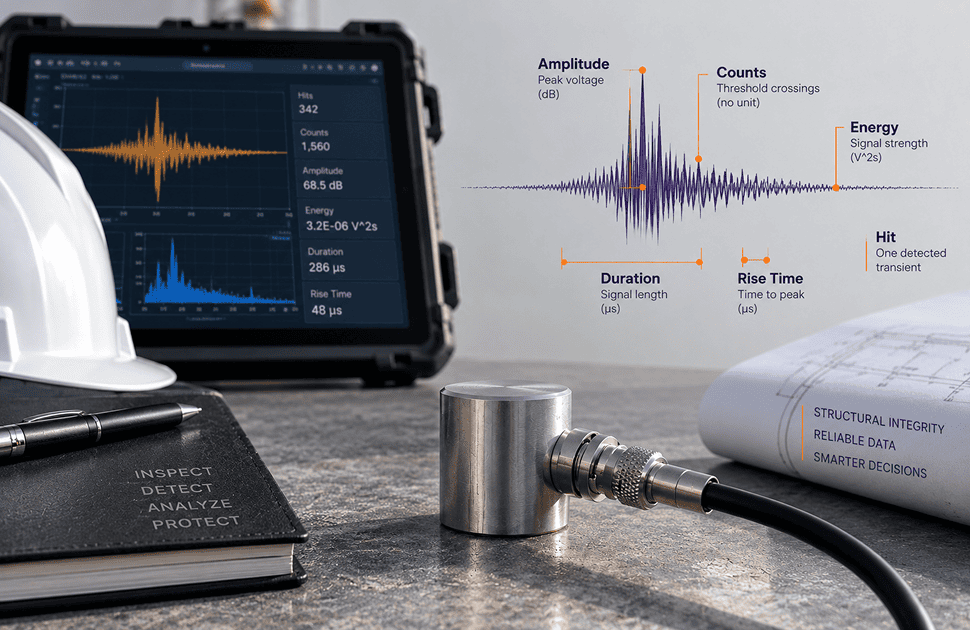
Every acoustic emission test is limited by one component more than any other. The instrumentation can be excellent and the analyst experienced, and none of it recovers information the sensor failed to detect.
ASTM E976 makes this point when explaining why sensor checks exist. Many things influence how sensitive a system is, but the sensor drifts more than any of them. Choosing the right one, mounting it properly and confirming it still performs are not preliminaries to a test. They largely determine what it can find.
How an acoustic emission sensor works
An acoustic emission sensor converts surface motion into voltage. The active component is a piezoelectric element, usually a lead zirconate titanate ceramic, which generates charge when mechanically strained. A stress wave from inside the structure displaces the surface by a fraction of a nanometre, the element deforms with it, and the resulting voltage is the signal.
Around it sits the rest of the assembly: a wear plate, often ceramic, protecting the element and transmitting motion into it; a backing material controlling how the assembly vibrates; a stainless steel housing giving mechanical protection and shielding against electromagnetic interference; and a connector carrying the signal out.
Two design choices in that assembly determine almost everything about how the sensor behaves.
The first is element size. Vallen Systeme's documentation sets out the relationship: element size governs where the sensor resonates, and shrinking it pushes resonance upward. Run that backwards and a low frequency sensor has to be physically large, which matters when access is tight.
The second is damping. An undamped element rings at its natural frequency, producing a large output at that frequency and very little elsewhere. Adding damping suppresses the ringing and flattens the response across a wider band, but the energy that was concentrated into the resonant peak is now spread out, so peak output falls. That single trade, sensitivity against bandwidth, is what separates the two sensor families.
Resonant sensors
A resonant sensor is deliberately left underdamped so that it responds strongly at one frequency. The result is high sensitivity within a narrow band and comparatively poor response outside it.
For most metallic structures this is the right compromise, and a sensor resonating near 150 kHz has become the default choice. Vallen positions its VS150-R that way in the catalogue, presenting it as a sensor that covers nearly the whole range of acoustic emission work and comes into its own on metallic pressure vessel integrity.
Lower frequencies serve different needs. Vallen's VS75 range resonates at 75 kHz, aimed at structures where signals travel a long way or through a lossy path, bitumen coated pressure vessels among them. The VS30 series drops lower again, with listed uses spanning tank floor corrosion and leaks, pipeline leaks, partial discharge and concrete. Lower still, the Physical Acoustics R1.5 resonates at 14 kHz, specified as useful between 5 and 20 kHz.
The pattern is consistent. Lower frequency gives greater range through attenuating material and larger structures, at the cost of admitting more mechanical and plant noise. Higher frequency rejects that noise but does not travel as far.
Broadband sensors
A broadband, or wideband, sensor is heavily damped to produce a comparatively flat response across a wide frequency span. Physical Acoustics describes its WD sensor as having a good frequency response over the range of 100 to 900 kHz. Vallen's VS45-H is documented with a peak at 280 kHz and a usable range from 40 to 450 kHz.
Flat is relative. Real wideband sensors ripple across their band, and a manufacturer's curve shows peaks and troughs rather than a straight line. What they offer is not a perfect response but a predictable one, where the recorded waveform reflects the arriving wave rather than the sensor's own ringing.
That matters for any work examining the waveform itself: frequency analysis, source characterisation, modal acoustic emission and crack mode classification. A resonant sensor imposes its own frequency on every signal it records, making frequency-domain interpretation unreliable. If you intend to analyse spectra, the sensor has to be broadband.
Reading a datasheet without being misled
This is where practitioners are most often caught out, and it is worth working through a real example.
The Physical Acoustics R15α is a widely used general purpose sensor. Its published specification lists peak sensitivity as 69 dB referenced to 1 V/(m/s), and simultaneously as minus 63 dB referenced to 1 V per microbar. It also lists two different resonant frequencies: 75 kHz referenced to 1 V/(m/s), and 150 kHz referenced to 1 V per microbar.
Both figures in each pair describe the same physical sensor. They differ because they are referenced to different quantities. Velocity referencing produces positive decibel values, pressure referencing produces negative ones, and the two references peak at different frequencies. The sensor's product name reflects the pressure referenced figure of 150 kHz, not the velocity referenced 75 kHz.
Three consequences follow, each a real source of error.
Comparing a sensitivity figure across manufacturers without checking the reference is meaningless. A positive number and a negative number may describe equally sensitive devices.
A stated resonant frequency depends on which reference is quoted, so two datasheets can disagree about the same sensor without either being wrong.
Figures that include an integral preamplifier are not comparable with passive ones. The R15I-AST, which contains a built-in preamplifier, lists peak sensitivity of 109 dB referenced to 1 V/(m/s). That is not a more sensitive element, but the same class of element with amplification folded into the number.
Bracketed values are referenced to 1 V per microbar, unbracketed to 1 V/(m/s). Figures come from published datasheets and should be confirmed against current versions before specification.
Variants worth knowing
Differential sensors. Two elements sit with their polarisation reversed relative to each other, wired into a preamplifier that responds to the difference between them. Interference arriving equally on both cancels, while the genuine signal survives. Physical Acoustics puts the benefit at roughly 2 dB over a single ended equivalent.
Integral preamplifier sensors. Vallen distinguishes active sensors, which contain a preamplifier, from passive sensors, which do not. Integrating the preamplifier reduces cable-borne noise pickup and simplifies installation, but it adds electronics inside the sensor housing, which restricts the temperature range.
High temperature sensors. Lead zirconate titanate loses its piezoelectric behaviour at a Curie point near 350 degrees Celsius, but the ceiling for sustained service sits well below that. Survey work puts the practical limit between 150 and 250 degrees Celsius, and that gap is why buffer rods and waveguides exist: they carry the wave out to an element sitting somewhere cooler. Lithium niobate holds its Curie point above 1100 degrees Celsius and supports sensors running at 500 to 600 degrees.
Preamplifiers and gain
Signals leaving the element are tiny and must be amplified before travelling any distance. Vallen's AEP3N preamplifier offers 34, 37, 40, 43, 46 and 49 dB, with an optional attenuator shifting the range down to between 0 and 15 dB.
That attenuator exists for a reason. Vallen cites proof testing of new composite pressure vessels as a case where sources are strong enough that gain must be cut to avoid saturation. More gain is not automatically better.
Mounting, coupling and verification
Mounting is covered by ASTM E650/E650M-24, which deals with what you couple the sensor with, what you bond or clamp it with, and the environmental conditions that bear on both choices.
The guide is explicit about what it does not replace, and the distinction is useful. It does not substitute for instrument calibration under E750, sensor recertification under E1781, or routine reproducibility verification under E976. Those are four separate obligations.
The calibration standards divide as follows. ASTM E1106 covers primary calibration of acoustic emission sensors and is the method manufacturers cite on their response curves. ASTM E1781/E1781M-20 covers secondary calibration, which is what periodic recertification uses. ASTM E976 is not a calibration standard at all. It asks a narrower question: does this sensor still respond the way it used to? Four situations call for it. Has the response drifted over time? Has the sensor been knocked about since it was last checked? Do the sensors sharing an array actually respond alike? And has anything changed after heating, cooling or a punishing environment?
Field verification uses the Hsu-Nielsen source, made by snapping a 2H pencil lead of 0.3 or 0.5 mm against the surface through a guide shoe. Vallen advises keeping the break far enough away that the distance exceeds twenty plate thicknesses, and choosing position by what you want to excite: breaking on the flat of the plate favours asymmetric modes, breaking centrally on the edge favours symmetric ones.

Choosing a sensor
Published research backs this directly. A review of sensor design observes that porous, directionally variable and viscoelastic materials all punish high frequencies, so dropping the sensor frequency preserves more signal against the noise floor. RILEM reaches the same conclusion for concrete from the other direction, recommending a few kilohertz to a few hundred kilohertz because anything past 1 MHz dies away too quickly to be useful.
Key takeaways
Resonant and broadband sensors are not better and worse versions of the same device. They sit at opposite ends of a deliberate engineering trade in which damping buys bandwidth and costs sensitivity.
Choose resonant when you need maximum sensitivity in a known frequency band, which covers most routine integrity work on metallic equipment. Choose broadband when the shape and spectrum of the waveform is the object of the analysis.
Above all, read the reference on any sensitivity figure before comparing it with another. A single sensor legitimately carries two very different sensitivity numbers and two different resonant frequencies, and treating those as interchangeable is the most common and most avoidable error in sensor specification.
Sources
- ASTM E650/E650M-24, Standard Guide for Mounting Piezoelectric Acoustic Emission Sensors, ASTM International: couplants, bonding agents, mounting fixtures, and the scope limitations relative to E750, E976 and E1781.
- ASTM E976-15, Standard Guide for Determining the Reproducibility of Acoustic Emission Sensor Response: stated purposes of sensor response checking.
- ASTM E1106, Standard Test Method for Primary Calibration of Acoustic Emission Sensors.
- ASTM E1781/E1781M-20, Standard Practice for Secondary Calibration of Acoustic Emission Sensors.
- ASTM E750-15(2025), Standard Practice for Characterizing Acoustic Emission Instrumentation.
- Physical Acoustics / MISTRAS Group published datasheets: R15α, R15I-AST, R15-UC, R1.5, R6, WD.
- Vallen Systeme, Acoustic Emission Sensors and Preamplifiers Description (2021) and Acoustic Emission Sensors Specification: element size and resonance, active versus passive sensors, AEP3N gain settings, application notes for VS150, VS75, VS30 and VS45 series, pencil lead break placement guidance.
- B. Tittmann et al., High Temperature Piezoelectrics: A Comparison, NDT.net: PZT Curie temperature and maximum recommended operating temperature, use of buffer rods and guided waves.
- Temperature Effects on Electromechanical Response of Deposited Piezoelectric Sensors, PMC6631685: lithium niobate Curie temperature and operating range.
- MEMS Acoustic Emission Sensors, review paper: frequency selection for porous, anisotropic and viscoelastic materials.
- RILEM Technical Committee 212-ACD recommendation, Materials and Structures (2010): frequency range guidance for concrete.